Investor Decisions Part 2: How to evaluate portfolio managers
Investor Decisions: How to evaluate portfolio managers
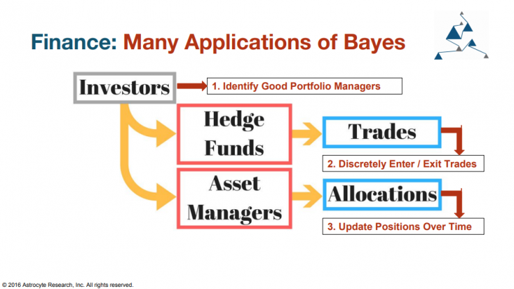
This talk first covers why using ‘Machine Learning in Finance is Hard‘ and then walks investors through three ways to apply Machine Learning and Science to:
- Evaluate Portfolio Managers
- Enter and Exit Trades
- Shift Factors and learn from your models’ failures
This talk and the sections below will briefly cover these topics.
Investor Decisions: How to evaluate portfolio managers
One of the key attributes of a modern portfolio manager is there ability to high risk-adjusted returns. Whether that is measured by a Sharpe, Sortino or, if you’re fancy, an Omega Ratio, the idea is that the larger the risks required to earn a reward, the more the reward should be penalized. Although this sounds great theoretically, these metrics are often difficult to use in practice, especially for strategies with limited track records. These reasons stem from the fact that metrics like the Sharpe Ratio are similar to a ‘t-distribution’ and have ‘fat-tails’. Meaning, using these measures alone, it is very hard to separate ‘Lucky’ from ‘Good’.
What is Lucky vs Good?
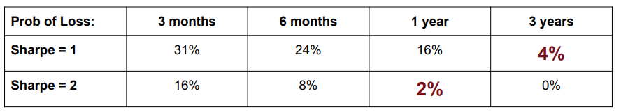
Some common target benchmarks for active managers stem are closely related to the average investment horizons of their investors. As a rule of thumb, I typically expect a good active manager at an Asset Manager to have a Sharpe Ratio (or Information Ratio if you’re being precise) of > 1.0 and a manager at a Hedge Fund to have a Sharpe Ratio > 2.0. The reason for this is that a manager with a Sharpe Ratio > 1.0 is expected to make money 96% of the time after 3 years. A Sharpe Ratio > 2.0 is expected to make money 98% of the time every year. If you work for a hedge fund and you are paid based on a ‘eat-what-you-kill’ model you’d like to be at least 98% sure you’ll be paid in a given year. For asset management firms with more patience and more balanced salary to bonus ratios, having solid returns on a three-year track record is the gold star you’re trying to achieve.
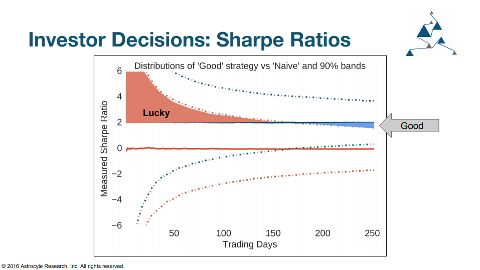
Understanding Lucky vs Good: Is my Sharpe > 2.0?
It is easy enough to calculate your Sharpe ratio for a given timeseries but the real question your investors want to know is whether you are more likely to have a 2.0 Sharpe or a 0.0 Sharpe. If it’s the latter, then they should withdraw their money and you should go back to the drawing board.
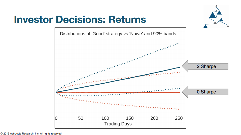
It can take almost a year to effectively seperate lucky vs good just by looking at returns (and assuming the same volatility)
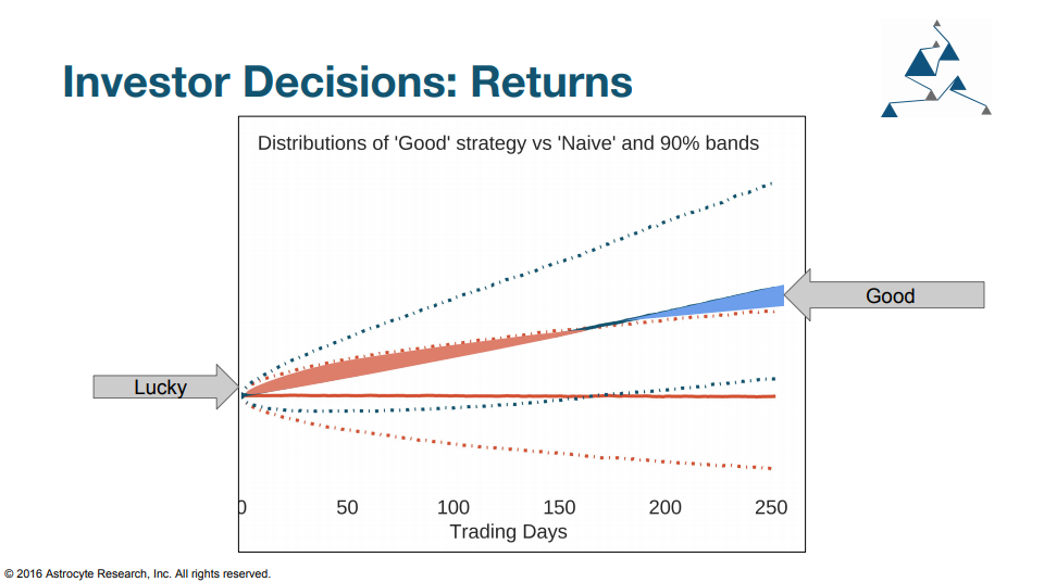
It is also true when looking at the distribution of Sharpe Ratios over time. In fact most strategies with high realized Sharpe ratios in the first 3 months are actually just lucky!
Classical Approaches to Evaluating a Portfolio Manager
Excluding other important factors like negligence, style drift, fees, etc… Let’s look at three metrics currently employed to track a PM’s performance:
- How much money have they lost in 1 day?
- How much money have they lost overall?
- What is my faith in their ability to continue to be profitable?
When you stop focusing on the performance measures, which as we showed above can be misleading, and instead focus on investor problem:
An investor in hedge funds wants to invest in as many 2.0 Sharpe strategies as possible and as few 0.0 Sharpe strategies as possible.
Therefore an investor can use the Bayes’ Rule and trailing performance data to update their probabilities for each investment.
Below is an illustration of this exercise. NOT INVESTMENT RECOMMENDATION. Use this as food for thought for your own research and not specific guidance for or against any investment.
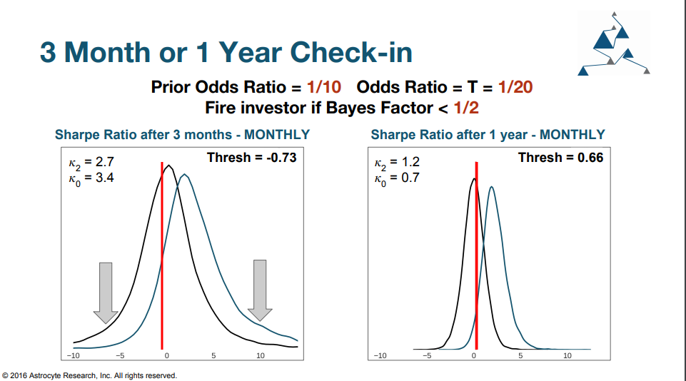
The above distributions show an investor who believed there was a 10% chance the PM had a 2.0 Sharpe ratio strategy (see Prior Odds Ratio = 1/10) and they wanted to be at least 5% sure that they are invested in a 2.0 Sharpe strategy (Odds Ratio = 1/20). If after 3 months (using only three data points) the Sharpe ratio was < -0.73 they should shut down the strategy (see disclaimer above). Likewise, the same could be said that after 1 year, they should exit the strategy if it only has a 0.66 Sharpe ratio.
Note this is contrary to the received wisdom of investment managers that like to ‘cut losers early’ and ‘let winners ride’. In reality you should ‘give losers some time’ and ‘cut winners if they haven’t won enough’
Trade Entry and Exit
Another type of investment decision that this bayesian approach can help improve is how to set ‘stop loss levels’. A stop loss is a rule-of-thumb that investors use as a signal when they should get out of a particular trade. Typically these rules fall into the following three categories: Fixed Loss, Daily Loss, Cumulative Loss over time.
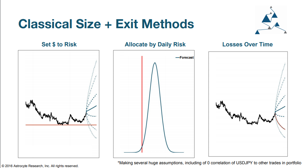
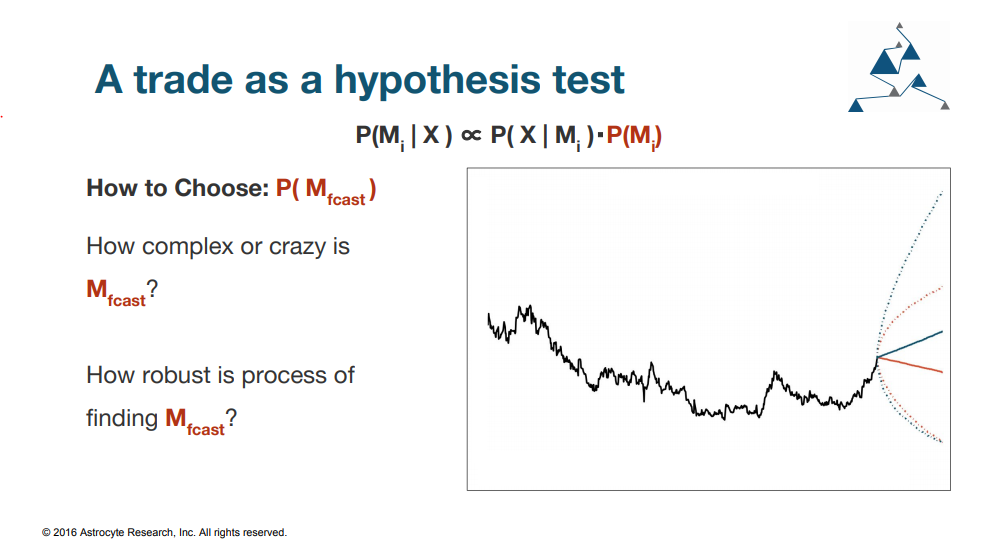
If you followed the previous section, you might guess that we say that these three methods are inferior to a rule that focused on testing the probability of being right vs the probability of being wrong in a given trade.
To use this approach you need to specify your prior beliefs and your confidence in your strategy vs another strategy. I typically either use what the market is pricing or what my risk models spit out as a generic alternative forecast to test my strategies against.
For those in the finance community, you aren’t typically that familiar with precision and recall curves when applied to trading. We can think of them as showing the relative tradeoff between type 1 and type 2 errors.
- Type 1 error: your trading idea is invalid but you haven’t hit your stop loss level yet.
- Type 2 error: your idea was right but you hit your stop loss. The latter example is often the most painful for traders as everyone hates having the right idea but not making money from it. Most people don’t even realize they make type 1 errors: who likes to admit to themselves that they were wrong but got lucky and made money on a trade.
We go on in the talk to show that by using the Bayes Ratio we can achieve higher Precision and Recall and minimize type 1 and type 2 errors better than other stop-loss strategies.
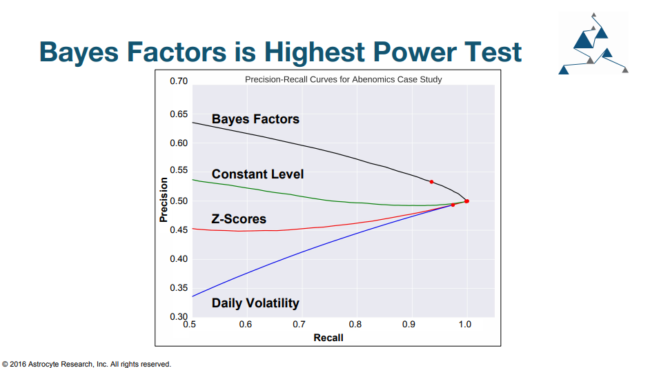
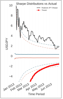
We show that a better stop loss level comes from looking at trailing Sharpe Ratios over time and deriving a curve based on your prior beliefs and your hull hypothesis. This maximized your probability of staying in a trade when you are correct and getting you out more quickly when you’re wrong. Here’s an example from the talk (using an Abenomics USDJPY example)
Factors as Investment Heuristics
When your models break you learn something
The end of this talk brings back together a framework for how humans and machines can work together in an investment framework. The key insight here is that all quantitative models based only historical relationships will inevitably fail because the structure of markets evolves.
Just think about how many quadrillions of interactions that occur within the real economy and markets that affect the pricing of the S&P500. How much confidence could possibly have in your simple model forecasting the SPY that just uses 1 variable: the P/E ratio?
Strong Opinions, Weakly Held - Paul Saffo
The goal therefore as a modern investor is to obtain thousands of high conviction empirical models that we call ‘Strong Opinions’ and produce a framework to adapt to their breaking down: We call this framework Breakpoints and have been using it since 2016 to forecast economic data, trends and correlations within global macro markets.